Econometrics Report

Author: Xiyao Huang

Ⅰ. Objective and Requirements of the Study

Facing the complex and changeable economic situation in today’s world, the total amount of exports, as one of the national economic indicators, is affected by many factors. “Industrial added value”, “RMB exchange rate”, “Interest rate”, “World GDP growth rate”, “China’s GDP growth rate” and other factors. I choose “the total amount of China’s exports” as the explained variable, “industrial added value”, and “RMB exchange rate” as the explanatory variable for the study.

By establishing econometric model and using the analysis method of time series analysis, this paper will analyze the main reasons for the differences in the total amount of China’s exports from 1994 to 2011, and the relationship between the total amount of China’s exports industrial added value and RMB exchange rate.

Ⅱ. Specification of Model

The total amount of exports (take out the inflation effect) was selected as the explained variable, the industrial added value and the RMB exchange rate were selected as the explanatory variable.

Founding a working file in Eviews, and select the data type as “Annual”. “Start Date” is set to“1994”, and “End Date” is set to “2011”. Inputting “Data Y X1 X2” in the command box of Eviews, and paste the data under the corresponding list of “Y X1 X2”.

Setting the model in the form of linear regression model, so I build an econometric model of the total amount of export：

Y=β0+β1*X1+β2*X2+e

Ⅲ. Data Collection

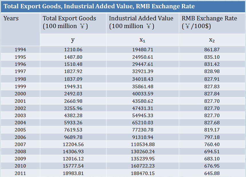
Ⅳ. Parameter Estimation

1. Scatter Graph

Inputting “SCAT X1 Y”, “SCAT X2 Y” in the command box to get:

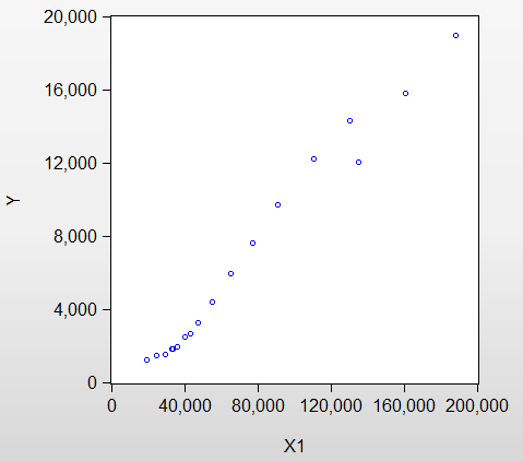
The figure above shows the scatter plot of the explanatory variable “Industrial added value” (X1) and the explanatory variable “Total amount of exports” (Y). It can be seen from the figure that most of the scatter points are distributed around a straight line, and it can be considered that there is a high linear correlation between X1 and Y.

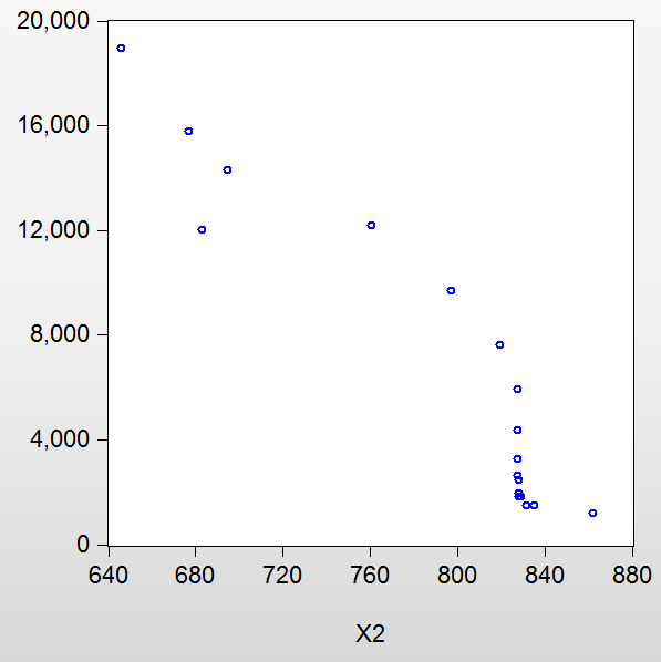
The figure above shows the scatter plot of the explanatory variable “RMB exchange rate” (X2) and explanatory variable “Total amount of exports” (Y). It can be seen from the figure that most of the scatter points are distributed around a straight line, and it can be considered that there is a linear correlation between X2 and Y.

2. Econometric Model：Y=β0+β1*X1+β2*X2+e

Enter "LS Y C X1 X2" in the command box to return the following regression results:

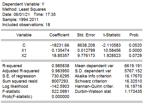
According to the data, the estimated result of the model is written as:

Y=-18231.6571069+0.135474045093X₁+18.8535713389X₂

(8638.216) (0.012799) (9.776181)

t=(-2.110573) (10.58454) (1.928512)

R²=0.985838 R²adjusted ̅=0.983950 F=522.0976 n=18

Ⅴ. Model Test

1. Test of Economic Significance:

Econometric Model：Y=β0+β1*X1+β2*X2+e

The model estimation results show that, assuming other variables unchanged, every 100 million RMB increase in the industrial added value will increase the total amount of export by 135.474 billion RMB on average.

Every 100 US dollars increase in the RMB exchange rate will increase the total amount of export goods by 1.8855348 billion RMB on average, which is consistent with theoretical analysis and empirical judgment.

Ⅳ. Parameter Estimation

Econometric Model：Y=β0+β1*X1+β2*X2+e

2.1 Goodness of Fit (R-squared)：

R²=0.985838 and the revised coefficient of determination R²adjusted ̅=0.983950 can be obtained from the data in the figure above, which indicates that the model has a good fit for the samples. The explanatory variable “Industrial added value” (X1) and “RMB exchange rate” (X2) are combined to explain the most explanations of explained variable “Total amount of exports” (Y).

2.2 F-testing

The null hypothesis is H0:β1=β2=0, and given the significance level is α=0.05. In the F distribution table, it can be found that the critical value Fα (2,15)=3.68 with the degree of freedom of k-1=2 and n-k=15. F=522.0976>Fα (2,15)=3.68 can be known from the above, and the null hypothesis H0:β1=β2=0 should be rejected. It indicating that the regression equation is significant, that is, the combination of “Industrial added value”(X1) and “RMB exchange rate”(X2) has a significant impact on the explained variable “Total amount of exports” (Y).

2.3 T-testing

The null hypothesis is H0:β1=β2=0, and given the significance level is α=0.05. From T-distribution table we know that the degree of freedom is n-k=15 and the critical value is 2.131. And β0, β1, β2 corresponding to the statistical distribution is t=-2.110573, 10.58454 and 1.928512, and their absolute values are all less than 2.131 except that β1 is greater than 2.131. It indicates that H0:β1=β2=0 should be accepted respectively under the significance level α=0.05. When other explanatory variables remain unchanged, “RMB exchange rate” (X2) has no significant effect on the explained variable “Total amount of exports” (Y).

When given significance level is α=0.05, since the T statistic corresponding to β1 is 10.58454, which is greater than 2.131, so the null hypothesis H0:β1=0 should be rejected. It indicates that at a given significance level α=0.05, “Industrial added value” (X1) has a significant impact on the explained variable “Total amount of exports” (Y).

However, when given the significance level is α=0.10, we can get the degree of freedom from T distribution table that is n-k=15, and the critical value is 1.753. In the corresponding T statistic distribution, β0, β1, β2 is t=-2.110573, 10.58454, 1.928512. They are all greater than 1.753. It indicates that H0:β1=β2=0 should be accepted respectively under the significance level α=0.05. When other explanatory variables remain unchanged, “RMB exchange rate” (X2) has a significant impact on the explanatory variable “Total amount of exports” (Y).

It can also be judged from the P value in the table that the corresponding P value of the estimated value of β1 is 0.0000, which is less than the given significance level. It indicates that at the given significance level, “Industrial added value” (X1) has a significant impact on the explained variable “Total amount of export” (Y). The corresponding P value of the estimated value is 0.0729, which is less than at a given significance levelα=0.10. It indicates that at a given significance level α=0.10, “RMB exchange rate” (X2) has a significant impact on the explained variable “Total amount of export” (Y).

Ⅵ. Conclusion

Through the above model test, the relationships between the “the total amount of China’s exports”, “industrial added value”, and “RMB exchange rate” are clearly shown. With the continuous upgrading and improvement of China’s industrial system, export volume of China will inevitably increase, and China’s economic influence in the world will continue to increase. It can be seen that the industrial system is like a major artery to a country’s economy. It is an indispensable foundation and a driving force for the vigorous development of the economy. While maintaining the stability of the RMB exchange rate, having a high-level industrial system is of vital importance to the breakthrough development of China’s economy.